Horse Racing Rumor Part 1: Can They Win AGAIN?
Introduction
After the horses win a race, can they win again in their next race? We would expect they have consistent performance but there are many factors affecting the outcome. For example, they have to compete with better opponents, or they may get tired, or luck, etc.
The above reasons are easily understandable while there are some mysterious saying existing without much data support:
- The horse in some stables are not able to perform consistently, i.e. they are less likely to win consecutively
- If the top jockey doesn’t ride the same horse again, they are likely to perform not as well as the previous run
- The odds of a previous winner is always higher than the odds of their previous race (for no reason)
This post will investigate how the performance of a previous winner is and disclose the myths. We will be using R and full script is available here
Loading the data
We will first load the library and the data sets. Actually they are the packages of tidyverse and the data is made public in Kaggle.
library(dplyr)
library(readr)
library(tidyr)
library(stringr)
library(ggplot2)

race_result_horse <- read_csv("../input/race-result-horse.csv")
race_result_race <- read_csv("../input/race-result-race.csv")
The data frame race_result_horse contains every horse record in the race but what we want in our analysis is only the winners. We can do this by a series of operation on our data frame.
race_result_horse_winner <- race_result_horse %>%
  # Remove records for rarely occured trainer, who are visiting trainers only competed in international race.
  group_by(trainer) %>%
  filter(n() > 20) %>%
  ungroup() %>%
  # We will ignore DH (Dead Heat) to ease analysis
  mutate(finishing_position = as.integer(str_extract(finishing_position, "[0-9]+"))) %>%
  # Sort the result by horse and race to allow lead and lag
  arrange(horse_id, race_id) %>%
  group_by(horse_id) %>%
  # Spawn lag lead for each column
  mutate_at(vars(-horse_name,-horse_id), funs(next_race = lead, prev_race = lag)) %>%
  ungroup() %>%
  # only take the record if the horse already ran its next race
  filter(finishing_position == 1 & !is.na(finishing_position_next_race)) %>%
  # Exclude those who are already in winning streak to reduce bias towards super horse
  filter(is.na(finishing_position_prev_race) | finishing_position_prev_race > 1)
First of all, let’s have a look at how they run next.
my_theme <- function(){
  theme(plot.title = element_text(hjust = 0.5),
        plot.subtitle = element_text(hjust = 0.5))
}

ggplot(race_result_horse_winner, aes(x=finishing_position_next_race)) +
  labs(title = "The position of the next race of winner", x = "position") +
  geom_bar() + theme_bw() +
  scale_y_continuous(expand=c(0,0), limits=c(0,200)) +
  scale_x_continuous(expand=c(0,0.1)) +
  my_theme()
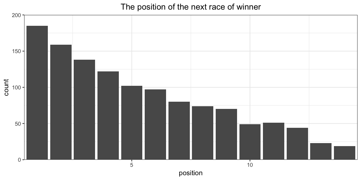
Actually winners generally run well in their next race.
Myth 1 - The horse in some stables are not able to perform consistently
But is that true for every trainer? Let’s look at it by each trainer. We recorded the position of the next race of winners and plot a bar chart. We will look at the proportion of each position instead of actual number for the sake of comparison. Also, we would like to compare with trainer’s overall performance.
We use grey color to represent the overall rank distribution and red for that of the winners’ next race.
# We will look at the proportion instead of actual number for the sake of comparison
race_result_horse_winner_by_trainer <- race_result_horse_winner %>%
  count(trainer, finishing_position_next_race) %>%
  mutate(total = sum(n)) %>%
  ungroup() %>%
  mutate(prop = n/total)

# compare with trainer's overall performance
race_result_horse_by_trainer <- race_result_horse %>%
  # We will ignore DH (Dead Heat) to ease analysis
  mutate(finishing_position = as.integer(str_extract(finishing_position, "[0-9]+"))) %>%
  filter(!is.na(finishing_position)) %>%
  count(trainer, finishing_position) %>%
  mutate(total = sum(n)) %>%
  ungroup() %>%
  mutate(prop = n/total)%>%
  # Remove rare occurance entry, who are oversea trainer
  filter(total > 10)

ggplot(race_result_horse_winner_by_trainer) +
  # plot a grey bar chart for overall performance
  geom_col(data=race_result_horse_by_trainer, aes(x=finishing_position, y=prop), alpha = 0.5)+
  # plot a red bar chart for winners' performance
  geom_col(fill = "red", aes(x=finishing_position_next_race, y=prop), alpha = 0.5)  +
  theme_bw() +
  # view by each trainer
  facet_wrap(~trainer) +
  labs(title = "The position of the next race of winner",
       subtitle = "Red - Winners, Grey - Overall",
       x = "finishing position", y = "proportion") +
  my_theme()
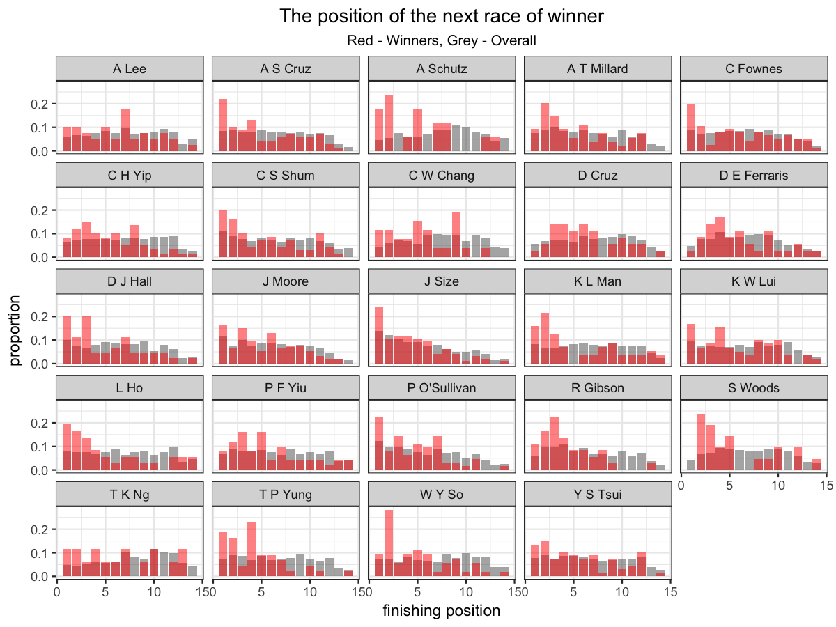
The more red area on top of grey area for top position, the better performance of the winner compared to the overall of trainer.
Most of the trainers have higher winning rate for previous winner and some even have 2-3x winning rate. Also, regarding the myth, it is true that some trainer has very few consecutive winner, e.g. D Cruz, D E Ferraris.
Myth 2 - Switching jockey = no confidence to win again?
Next, we will tackle the second myth and we will look at whether switching jockey will affect performance of winners.
We use red to indicate switching jockey and blue to indicate same jockey.
# We will look at the proportion instead of actual number for the sake of comparison
race_result_horse_winner_by_jockey <- race_result_horse_winner %>%
  mutate(same_jockey = ifelse(jockey == jockey_next_race, "same", "different")) %>%
  count(jockey, same_jockey, finishing_position_next_race) %>%
  mutate(total = sum(n)) %>%
  ungroup()  %>%
  mutate(prop = n/total) %>%
  group_by(jockey) %>%
  # Ignore less occurence jockey
  filter(sum(n) > 20) %>%
  ungroup()

ggplot(race_result_horse_winner_by_jockey) +
  geom_col(aes(x=finishing_position_next_race, y=prop, fill = same_jockey),
           position = "identity",
           alpha = 0.5) +
  theme_bw() +
  facet_wrap(~jockey) +
  labs(title = "The finishing position of the next race of winner",
       x = "finishing position of next race", y = "proportion",
       fill = "Same/Different jockey") +
  my_theme()
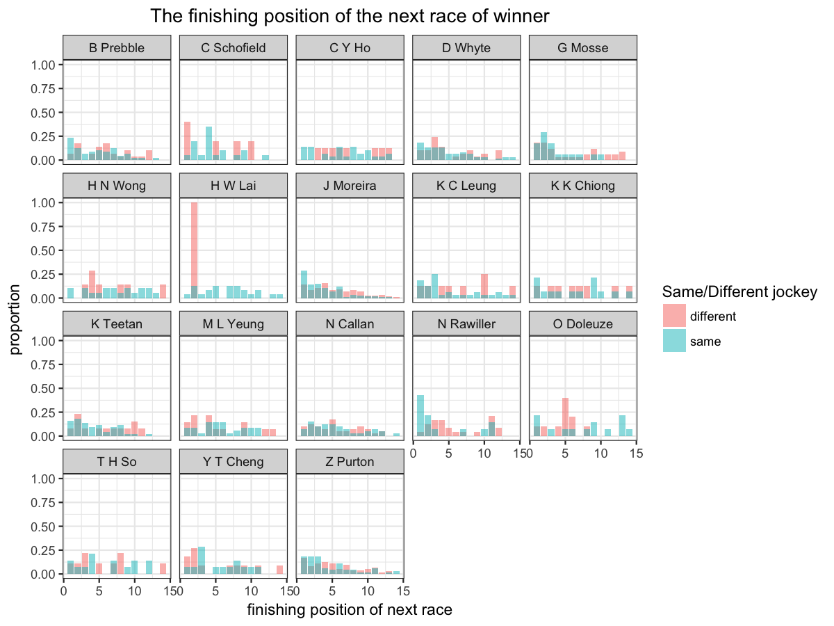
Although the data for some jockey is limited, we are still able to see some insight. There are jockey who ride the same horse again and perform well. On the other hand, there are some jockeys, such as Z Purton, performed the same with other jockeys for his previous winner. The myth only holds for some jockeys such as J Moreira and N Rawiller.
Myth 3 - Odds goes up after a win?
So, it comes to the last myth - The odds of a winning horse is usually higher in their next race.
We will look at the number of times the odds increased or decreased in the next race, by each jockey.
race_result_horse_winner_odds_by_jockey <- race_result_horse_winner %>%
  mutate(same_jockey = ifelse(jockey == jockey_next_race, "same", "different")) %>%
  select(race_id, horse_id, win_odds, win_odds_next_race, jockey, same_jockey) %>%
  mutate(change = ifelse(win_odds_next_race > win_odds, "up","down")) %>%
  group_by(jockey) %>%
  filter(n() > 20) %>%
  ungroup()

# Odd change
ggplot(race_result_horse_winner_odds_by_jockey, aes(x=same_jockey)) +
  geom_bar(aes(fill = change)) +
  theme_bw() +
  facet_wrap(~jockey) +
  labs(title = "Change of odds in the next race of winner",
       x = "Same/Different jockey", y = "Count",
       fill = "Odds change") +
  my_theme()
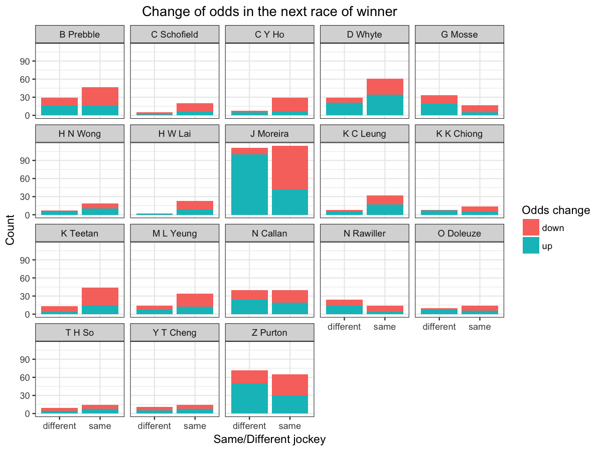
When the horses switch jockey, the odds will go up most of the time, especially for the horse won by J Moreira. On the other hand, it is quite balanced if the horse is ridden by the same jockey.
Summary
Most winning horse can maintain consistent performance in their next race. It seems jockey and trainer is two of the factor affecting their performance from above analysis.
However, within each trainer/jockey, their could be many other factors. I will leave it to the reader to do further analysis. For example, does the odds reflected the performance? Is the performance vary for each class / horse rating?
Enjoy!
The code for this analysis is available here